A Complete Guide to Open Addressing & its Classification to eliminate Collisions

Hashing has the fundamental problem of collision, two or more keys could have same hashes leading to the collision. Open addressing also called as Close hashing is the widely used approach to eliminate collision. The idea is to store all the elements in the hash table itself and in case of collision, probing (searching) is done for the empty slot.

Before reading this post, please go through the following posts,
– Intro to Hashing
– Separate Chaining and its implementation

Load Factor:

Load Factor denoted by α is the measurement of how well elements in the Hash Table are distributed. It is defined as,

                       No. Of stored elements in the table
Load Factor (α) =   __________________________________________ = n/m    
                     Capacity(or size) of Table at the moment

We’ve already seen it w.r.t. Separate Chaining,
LOAD FACTOR will be different in the context of Open Addressing. Under open addressing, no elements are stored outside the table, i.e. no chain(linked list). All elements have to occupy in the table itself. Therefore, as a result number of elements in the hash table will never exceed the capacity or we can say LOAD FACTOR will be at max one.
Say n = 5 elements and m = 5 slots, then, α = 1 . It says that hash table is completely filled.
For n = 3 elements and m = 5 slots, then, α = 0.6 . It says only 60% of the hash table is filled.

Classification of Open Addressing:

The time complexity of whereas operations in open addressing depend on how well, probing is done or in other words how good the hash function probes on collision. Based on this, there are 3 classifications of Open Addressing.

1. Linear Probing:

Say h(Element) is the hash function, then function under linear probing will be as,

h’(K, i) = (h(K)+i) mod m

Where m is the table size and i = 0, 1, 2, ….., m-1 and K for Key of the Element and h(K) is the ordinary hash function. So, our hash function under linear probing becomes h’(K, i) and h(K) is now referred as Auxiliary function.
Let’s try to understand with an example, In the shown table, we require to store 82 and size of table is 10. Our auxiliary hash function is (Element) mod 10, i.e. computation will be done as followed,

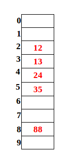
h’(82, 0) = (h(82)+0) mod 10 = 2 mod 10 = 2 ; collision as index 2 already filled. So i becomes 1
h’(82, 1) = (h(82)+1) mod 10 = 3 mod 10 = 3 ; again collision, i = 2
h’(82, 2) = (h(82)+2) mod 10 = 4 mod 10 = 4 ; again collision, i = 3
h’(82, 3) = (h(82)+3) mod 10 = 5 mod 10 = 5 ; again collision, i = 4
h’(82, 4) = (h(82)+4) mod 10 = 6 mod 10 = 6 ; No collision.
Hence, element 82 will be stored at index 6.

Drawbacks associated with linear probing:

Drawback1:
For lookup operation, if we get an empty slot means the element is not present. Consider the following scenario, in the above hash table,
-insert(34)
-delete(35)
-search(34)

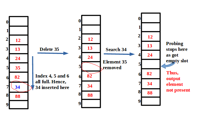
Thus, even though element 34 present in the table, yet got not present.
The Solution to this problem is to designate some constant element, say ‘D’, for every deletion. Now, look up operation won’t stop until an empty slot is not found. During insertion operation, ‘D’ will be considered as empty. This solution will be applied to all kinds of open addressing.
Drawback2: Primary Clustering
Linear probing does probing on each slot one by one in a circular manner. In the above example, what if all the slots are filled except slot 9. Now element 100 is required to store. Probing will be done for i = 0 to i = 9 and that’s the size of the table. The time complexity is no longer constant even for the lookup operation. This is referred as Primary Clustering. Solution: Quadratic probing

2. Quadratic Probing:

Linear probing probes each slot linearly i.e. one by one each slot in a continuous manner. Now, however, the interval between probes will be quadratic rather than linear.
h’(K, i) = (h(K) + C₁i + C₂ i²) mod m
See the following,

Drawback: Secondary Clustering
All the probes done for an element is referred as Probe sequence. Such as an example shown in Fig2, probe sequence of element 82 is 2, 3, 4, 5, 6, and so on. If multiple elements generate the same hashes, then, their probe sequence will be same. As a result, there’ll be again, clustering of elements. h’(K₁, 0) = h’(K₂, 0) implies h’(K₂, i) = h’(K₂, i)
Also, C₁, C₂, and m have to be chosen wisely to make full use of the hash table. That’s a constraint here.
Thus, both linear and quadratic clustering is prone to secondary clustering.

Solution: Double Hashing

3. Double Hashing

Clustering rises because next probing is proportional to keys, that’s why got the same probe sequence. Double hashing makes use of another different hash function for next probing. As a result, probe sequence will become random.
h’(K, i) = (h₁(K) +ih₂(K)) mod m

This is most widely used, as it has no major drawbacks.
Cons of Double hashing:
1. Take comparatively more time in computation
2. Complex Implementation

Knowledge is most useful when liberated and shared. Share this to motivate us to keep writing such online tutorials for free and do comment if anything is missing or wrong or you need any kind of help.

Keep Learning… Happy Learning.. 🙂

Recommended -